Artículo de investigación
Agricultural Production Conditions in Boyacá
Las condiciones de la producción agropecuaria en Boyacá
Helmuth Yesid Arias Gómez*
Gabriela Antošová**
* Economist. Ph. D. in Applied Economic Analysis and Economic History. Affiliation: Masaryk Institute of High Studies. Czech Technical University in Prague (Czech Republic), ariashel@cvut.cz https://orcid.org/0000-0003-0107-8611
** Ph. D. Social and Regional Development. Affiliation: Academy of Humanitas in Sosnowiec (Poland) gabriela. antosova@humanitas.edu.pl and College of Applied Psychology, antosova@vsaps.cz. (Czech Republic). https://orcid.org/0000-0001-5330-679X
Cómo citar: Arias, H. Y., & Antošová, G. (2024). Agricultural Production Conditions in Boyacá. Apuntes del Cenes, 43 (77). Págs. 243-269. https://doi.org/10.19053/uptc.01203053.v43.n77.2024.16304
Fecha de recepción: 29 de julio de 2023 Fecha de aprobación: 3 de diciembre de 2023
Abstract:
This article uses data from the Census of Agriculture 2014 pertaining to the Department of Boyacá. It connects the production performance at the municipal level to a set of rural determinants, which encompass the exploitation of the agricultural potential. This approach highlights features of the agricultural sector in Boyacá: the predominance of annual crops, the break-up of agricultural units, the family arrangements to supply labor input, and the lack of a widespread export stuff, inter alia. The methodology employs a spatial approach that seeks to identify spatial patterns in the agricultural output, using the municipality as the spatial unit. We resort to spatial econometrics to model the determinants of the agricultural output, and to point out a better spatial structure according to the pool of data. The econometric results confirm a kind of spatial dependence in the error, suggesting the influence of common shocks affecting the agricultural output, everywhere the municipalities of Boyacá. Throughout the region, the traditional production profile, based on annual crops to satisfy the national consumption, prevails. This type of production depends on typical rural conditions: small plots of land, little mechanized production, family work and precarious wages.
Keywords: census of agriculture; agricultural production; production structure; spatial interaction; spatial econometrics; Colombia.
JEL Classification: R12; R14; R58; C51; N56.
Resumen:
El artículo se inspira en los resultados del Censo Agrícola 2014 para Boyacá. El propósito es relacionar el desempeño puramente productivo con los determinantes de economía campesina que sirven de contexto a la producción en toneladas. Entre estos últimos se destacan la especialización en cultivos transitorios, la fragmentación de las unidades de producción agrícolas, la provisión familiar de trabajadores, la ínfima importancia de la oferta exportable, etc. La metodología adopta un enfoque espacial que persigue identificar los patrones espaciales de la producción, definiendo el municipio boyacense como la unidad de análisis en el plano geográfico. La econometría dilucida cuál es la mejor estructura en el espacio que modela los datos básicos. De esta manera se convalida el modelo de error espacial, que da lugar a la presencia de shocks comunes a todos los municipios boyacenses, afectando en todos ellos la producción agrícola. La interacción entre dichas unidades geográficas permite modelar la producción volcada mayoritariamente hacia el mercado nacional, la cual es explicada significativamente por determinantes típicamente rurales: la fragmentación de las unidades agrícolas, las técnicas de producción escasamente mecanizadas, la relevancia del trabajo familiar como factor de producción, y las precarias remuneraciones.
Palabras clave: Censo Agrícola; producción agrícola; estructura productiva; interacción espacial; econometría espacial; Colombia.
INTRODUCTION
The driving force behind rural underdevelopment and general agricultural backwardness is the gap between rural and urban wages, as well as the widespread structure of land ownership and tenure, which leads to an acute concentration of vast extensions of land in a reduced number of plots. On the other hand, the production of some commodities, such as potatoes, coffee, onions and tomatoes, is dominated by the fragmentation of countless small farms, which limits economies of scale.
To analyze this complex reality, we use the available sectoral information contained in the 2014 Census of Agriculture, which provides a valuable basis for a comprehensive study of production, technology, land use and tenure, and the social realities of the rural sector. Subsequently, the data pool provides the opportunity for further analysis and modeling. In fact, it has become the source of further research on the rural production profile or rural social conditions. (Fedesarrollo, 2019; Rojas, 2019).
The Census of Agriculture data for Boyacá reflect the conditions of a predominantly agricultural region that has been sociologically shaped by rural activities. Fifty-five years have passed since the last Colombian Census of Agriculture, and since then society has obviously demanded an update on the diverse aspects of the rural sector. In this way, the information gap has been filled, addressing the diagnosis of the real conditions in the countryside and providing the data inputs for decision making, analysis and interpretation.
The timely contribution of the Census of Agriculture includes the full coverage of rural areas, and the disparate nature of the data collected during the operational strategy. For our purposes, we will work with the available municipal data on production, land tenure and production units. There is an explicit interest to inquire on this information to reconcile the production measured in tons, the predominant land tenure, the extension, and the number of production units, in order to empirically contrast the relationship between production and rural conditions.
This article aims at provide a spatial reading of the Census of Agriculture information zooming in on data at a municipal level, to reflect spatial trends in production. We highlight the most relevant areas in terms of production, while making a spatial and conceptual overlap with other related aspects of the geography and the natural surroundings.
The content of this article is divided into three parts. The first part presents a rough outline of the general conditions that are common to rural exploitation in Boyacá. The second part describes the production profile, considering the individual relevance of the 123 municipalities according to the production reported by the Census of Agriculture. The following empirical section forms the core of the article, combining a spatial description of the agricultural production and a model run of spatial econometrics Finally, the last section concludes the analysis. The contribution of the article lies in the use of census information and the empirical application to Boyacá. It is hard to find this kind of research elsewhere, using the comprehensive baseline data provided by the Census of Agriculture.
The Census of Agriculture revealed information about the traditional dual structure of land ownership. There is an acute concentration of larger properties, and a break-up of small production units. At a general level, the results confirm the fragmentation of the units of exploitation; taking into account for the whole country, 70.4% of the Agricultural Production Units (APU) had an extension inferior to 5 ha. Although the share of this group of small exploitations in the total surface of the APUs is minimal, just 2%, on the other hand, the production units larger than 1,000 ha represent only 0.02% of the total of the units of agricultural production.
It gave rise to the hypothesis of a greedy interest in speculation as the driving force behind the intensification of land concentration. (Suescún, 2013). This also showed a kind of under-utilization of larger plots of land, preferentially dedicated to cattle raising. The consequences for the production arrangement are pointed out by UNPD (2011) which defines a dual structure of agrarian exploitation in which, the huge extensions concentrate on cattle raising or on unproductive purposes. Conversely, there are countless small family plots where labor relations are based on non remunerative labor. This uneven structure also raises several concerns about the appropriate use and exploitation of land, as it leads to clear conflicts between the use and the potential of land.
In fact, in the midst of this duality, a stubborn shift in the Colombian specialization was underway, a transformation that favored the perennial crops based on the extensive exploitation of large farms, whose management is in charge of the agribusiness and commercial agriculture. After the agricultural liberalization reforms that had been introduced, the emerging commodities linked to the agribusiness (sugar cane, oil palm, rubber) underwent a remarkable expansion, fueled by the mobilization of the international capital. This series of perennial crops requires large plots of land capable of favoring the exploitation of economies of scale, as a condition of profitability (Suescún, 2013).
Confirming the post-liberalization trend, perennial species continued their expansion and became the most extensively cultivated species, reaching 74.8% of total. The current dominance of perennial crops demonstrates the continuous disclosure of competitive advantages in the national agriculture (Machado, 2015).
On the other hand, the important role of small APUs and the family production is relevant in the context of the Colombian analysis of agricultural productivity, and the rural sector specifically in the higher lands of the cordilleras. The concern about the economic performance in small-scale exploitations gave rise to the concept of the "inverse relationship" as a stylized fact dominating the sectoral efficiency (Barret et al., 2010; Berry, 2017). In this sense, small farms tend to have higher returns to land use than large farms. However, in terms of labor productivity, small farms show lower efficiency, mainly due to the scarce capital endowment and precarious technical conditions.
The reasons for higher land yields are based on the need to exploit commodities with high value per hectare (vegetables, coffee) and to absorb the availability of family labor (Berry, 2017). This argument can be contrasted with the high efficiency of large agribusinesses, an activity based entirely on economies of scale. Other motives for discussing the "inverse relationship" emerge when considering the concentration of markets and soil quality aspects (Barret et al., 2010). Moreover, after having evaluated the small farms by means of a more comprehensive set of determinants, the dimension of land is complemented by the fertility, the condition of the crop, the climate, the technology and, of course, the involvement of complementary factors of production.
In this regard, the low diffusion of technology and mechanization represents a remaining concern for improving the efficiency of small farms. In this context, few producers have had access to the credit system, which reinforces the idea about the general limitations to the implementation of modern technological frameworks, for the greater part of the agricultural sector. The divergence in terms of productivity and factor use has already been pointed out by Fedesarrollo (2019), whose estimates show a lower use of labor in agricultural tasks depending on the size of the plot.
In fact, in smaller APUs, the average is 1.9 permanent workers per ha, and in larger land units, the average is 1 permanent worker per 100 ha.
In addition, the census highlighted the current use of the land, with the aim of assessing its true production potential. In Colombia, 25 million hectares are suitable for agriculture, but only 25% are used for this purpose. Conversely, the land suitable for livestock production corresponds to 16 million ha, but the effective area for livestock is 24.8 million ha (Fedesarrollo, 2019). This conclusion demonstrates the mismatch between the natural endowment and the effective use of land, raising concerns about suboptimal production results, and the negative impact in terms of sustainability.
The conditions revealed by the census results can be verified by other sources of information (household surveys, unemployment surveys). It is generally accepted that there are significant gaps between urban and rural social conditions and development potential. At the national level, about 80% of the rural population has attained up to a secondary education level. Regarding the rural labor markets, they are characterized by specific precarious conditions, but in the strict sense unemployment is not really a predominant burden for the rural sector, because family exploitation keeps potential workers at home. However, the most ominous social condition is the low remuneration and the widespread practice of absorbing family members under a regime of non remunerative labor (Rojas, 2019). Nevertheless, the prevalence of this type of arrangement is not a general rule and depends on the crop class. For example, in the context of agribusiness and commercial exploitation, a more modern system of labor absorption predominates, which results in a more extended wage relationship (Suescún, 2013).
PRODUCTION PROFILE AND NATURAL ENDOWMENTS
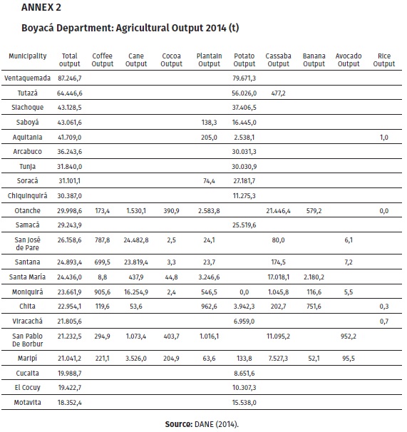
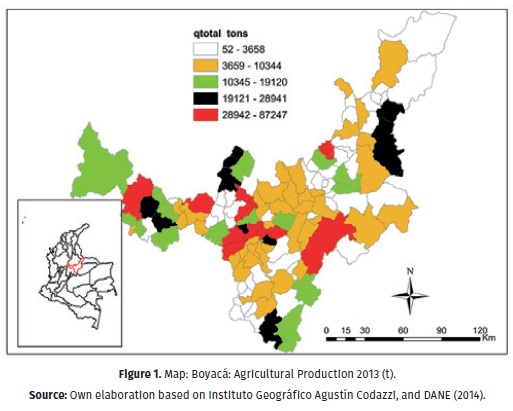
The bulk of production in Boyacá is based on annual crops, namely: potato, tomato, onion, carrot, and others. Among the perennial crops, the following are predominant: sugarcane, pear, plantain, blackberry, orange, plum, and apple (CGIAR, 2021). In the national ranking, Boyacá is the first producer of onion and tomato, and the second in potato production. Its role is relevant in the production of fruits and milk. Figure 1 and Annex 2 show the main agricultural producers and present the analysis of a diverse set of production conditions, driven by the principle of comparative advantage, where cost differences and productivity explain specialization. The diversified supply includes typical products of cold countries: potato, onion, tomato, carrot, corn, pea, bean, but also mild climate crops such as sugar cane, plantain, casaba, and a wide range of fruits.
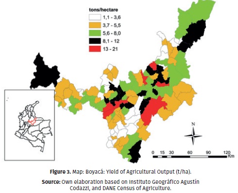
The main producers of annual commodities tend to be more productive, specifically when they appear on top of the list according to the agricultural yield. Potato producers tend to have a better yield given climate conditions and geography. Using the updated information, CGIAR (2021) asserts that the yield in potato has evolved positively in the recent periods, increasing from 13 t per ha in 2015 to 17 t per ha in 2021.
The surprising results in terms of potato production reveal the role of some municipalities such as Saboyá and Chíquiza. In fact, the leading agricultural municipalities are potato producers: Ventaquemada, Tutazá, Siachoque, Arcabuco, Tunja and Soracá. On the other hand, Aquitania excels in the production of onion. In the production of cane, the following three municipalities stand out: Moniquirá, San José de Pare and Santana. Coffee crops appear in mild areas of Moniquirá, San José de Pare, Santana, Zetaquira, Buenavista, Miraflores, Berbeo, San Pablo de Borbur and San Eduardo, even if the scale of production is rather moderate. (A detailed scheme is shown in Annex 2).
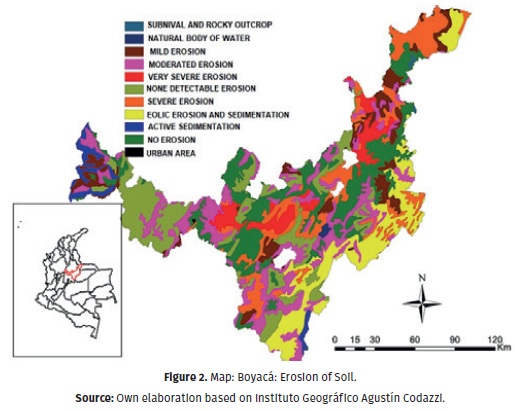
Figure 2 shows an interesting contrast between the soil conditions and the main producers of agricultural commodities, and therefore the conclusions show an obvious overlap of the most productive areas and better soil conditions. Conversely, the most affected areas with the most degraded soils coincide with the desert of La Candelaria. This area, which is shared by the municipalities of Villa de Leyva, Sáchica, Sutamarchán and Tinjacá, has little agricultural activity and is characterized by tourism and pottery. In the department of Boyacá, the best land is dedicated to the production of cold climate products, and ends up as the most productive place.
In terms of agricultural specialization, soil conditions and geography shape the production profile in a neat Ricardian vein. Figure 2 shows the support for the exploitation of agricultural endowments and the deployment of crops across the territory. Accordingly, the economic theory shows that a more enduring explanation of production specialization is rooted in costs and productivity differentials due to Ricardian comparative advantage.
The census provides information on the universe of production units in terms of aspects strictly related to production, but also in terms of land ownership, land use and cultivated areas. The information confirms the relevant role of Boyacá as an important producer of some crops, specifically in annual species, while the department's role in the perennial products is rather modest.
Boyacá is an agriculture-specialized department and competes with the other regions for the leading role in production and area. Boyacá's share of agro-industrial products1 is only 2.7% at the national level, and 3.3% in terms of total area and number of production units. Its role is more significant in the national comparison of cultivated area for products such as sugar cane (8.1%) and tobacco (6.6%). In the case of fruit production, its share is 5.2% at the national level and 4.8% in terms of the number of production units.
In addition, Boyacá seems to be a prominent producer in the category of plantains and tubers, accounting for 3.9% of the national cultivated area and 3.8% of the number of production units. If potato production is singled out, the real dimension of the department's importance is increased due to its cultivated area (20.7%) and the number of production units (21.5%). The typical small-scale dimension of potato production is emphasized everywhere, more precisely, 95% of the production units correspond to extensions of 3 ha or less; at the same time, 4% or less of the individual producers belong to some kind of associated scheme for the commercialization of this commodity (CGIAR, 2021).
The production profile has led to the identification of chains that include the positioned annual crops, but also some perennial commodities distributed throughout the region. This means that the public policy has prioritized a set of production bid in line with the comparative advantages spurred by the geography. The list is as follows: potato, onion, carrot, quinoa, pea (annual crops); sugar cane, coffee, cocoa, blackberry (perennial crops) (CGIAR, 2021)
Land Ownership and Farm Size
This article benefited from the availability of the data disclosed by the Census of Agriculture, considering that land ownership and farm size showed a clear relationship with yield and rural welfare. In the analysis of economics of development, the concept of "inverse relationship" is typically applied, defined as the highest yields achieved by the small rural properties compared to the extensive rural exploitations. The driver of this stylized fact is the productivity of labor, and the intensive exploitation of the unit of labor, to the extent that a small farm is exploited by a familiar unit making the land more productive. On the other hand, the large extensions of land receive lower yields per unit of land. This argument has been widely explored in Colombia by Berry (2017), and has been discussed elsewhere (Barrett, 2010).
However, despite the "inverse relationship", the opposite logic applies when analyzing the productivity of labor. In the latter case, extensive large-scale exploitation demonstrates higher labor productivity because it relies on the widespread application of technology and capital.
In Boyacá, agricultural exports are rather scarce, and most of the regional production is sold in the domestic market, mainly in the main cities of the country: Bogotá, Bucaramanga, and Barranquilla. In our spatial econometric analysis below, we have included a proxy for the importance of national markets, measured by the linear distance from the municipal centroids to Bogotá. This production profile in Boyacá is relevant for the future performance of the regional agricultural sector, taking into account a better performance of the crops engaged in export activities, in terms of a more efficient use of labor and equipment, higher specialization, more extensive own land tenure, and more frequent technical advice (Fedesarrollo, 2019).
In this region, the production system based on small farms, typical of the higher mountain areas, predominates. Accordingly, the information at the national level for Colombia indicates that the greater number of APUs is concentrated in the Colombian Andean region, and 45% of them belong to Boyacá, Antioquia, and Cundinamarca. Otherwise, in the flatter areas of Colombia, the regime of land use is more extensively applied to large farms (Rojas, 2019).
EMPIRICAL STRATEGY
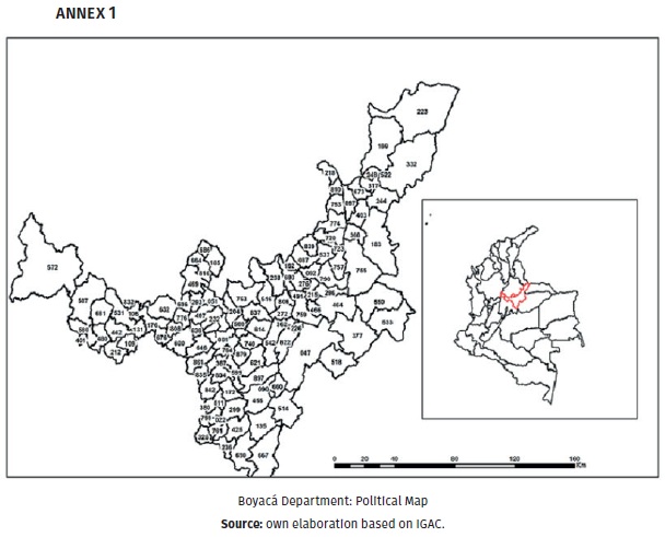
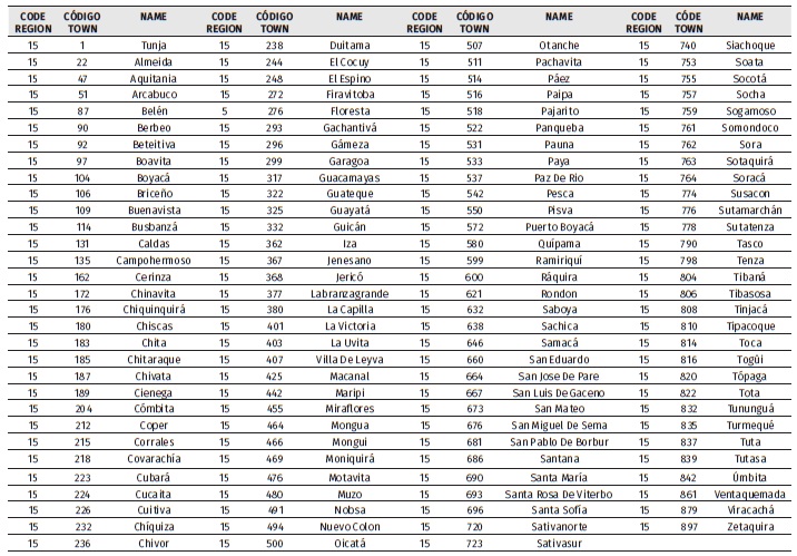
To give local relevance and a spatial focus to the analysis, we run a spatial econometric model applied to the rural production measured in tons. The data set covers 123 municipalities in Boyacá, thus providing a rich representation of rural conditions and production characteristics. The data sources are DANE's2 Census of Agriculture, and the geographic support and layers are drawn from IGAC3. The sources provide a consistent database which considers suitable attributes of each municipality, and simultaneously, the geographical support for introducing the geospatial dimension of the research. The scripts dealing with the econometric modelling have been performed in the R software, and for the cartographic deployment we used the ARCPRO software. Appropriate procedures of spatial econometrics have been followed to deal with spatial interaction and spatial structure of data, applying standard procedures following the pioneer text of Anselin (2001), and the recent recommendation of Elhorst (2010).
The 123 municipalities that make up the department of Boyacá are assumed the primary spatial unit of the analysis. The existing production and demographic information are duly attributed to each municipality, and the level of detail is sufficiently specific to undertake a spatial analysis, and to specify the econometric model. The spatial approach is the driving force of the analysis because we expect that geographical proximity determines common production and rural characteristics across geographical units.
The econometric specification aims at find a spatial approach more suitable for modelling agricultural production, as described by the Census of Agriculture, using as arguments the most meaningful information in the data pool, attributed to the characteristics of the Colombian rural context. Most of the variables are taken from the census reports, a common source that explains the common coherence of the data. On the other hand, the source for the Unsatisfied Basic Needs (NBI) is the periodic measurement developed by DANE.
The NBI became a relevant indicator of the rural conditions to the extent that the multi-dimensional poverty in the rural sector doubles the urban indicator. One salient feature disclosed is the percentage of rural workers (66.6%), belonging to a very small number of APUs, a fact that asserts a wide incidence of poverty (Machado, 2015).
DANE provides population projections at the local level and publishes annually the statistics about poverty, specifically in the rural context. It uses social conditions and demographic determinants for the production. The local population is relevant because it represents either the size of the local market, or the local availability of labor that can potentially be embedded in the rural tasks. Typically, the population incorporates the size of local markets and acts as a proxy for demand linkages that contribute to strengthening the scale of production.
The spatial econometric model runs the interaction of a set of exogenous variables that turn out to be determinant in agricultural production. Throughout this article we surpass the definitive contribution of the Census of Agriculture for updating the pool of data available to researchers, because the Census findings make the coverage of the rural reality complete, and make the data set mutually compatible.
From the Census of Agriculture , we obtain the number of agricultural production units (APUs) and the percentage of owners according to the land tenure system. Both categories provide relevant information about the particular conditions on the ground that affect production, namely: how fragmented the structure of rural exploitation is, and how land ownership can motivate the family economy to strive to make the agricultural projects more productive.
As long as the space is a real concern in our research, the variable "distance" measures the geographical proximity to Bogotá as the most relevant market for the agricultural production of Boyacá. The distance, measured as linear distance between the 123 centroids and the national capital, is calculated using geostatistical tools. This approach seems really surprising, since the majority of Boyacá's production is intended to satisfy the national market, and according to the traditional typologies, this type of non-tradable production predominates around the proximity of the main national urban cores (Fedesarrollo, 2019).
The spatial intuition implicit in this measure of distance is based on the more intense spatial interactions fostered by geographic proximity. This approach is consistent with Tobler's law, which states that the nearby things appear more related than distant things, and confirms the stylized fact that the process of overcoming space is costly, and economic rationality demands that such costs must be minimized (Osland, 2010).
Elhorst (2010) suggests including additional spatial interactions to capture the true process of spatial interdependence between endogenous, exogenous, and omitted exogenous variables in the model.
The next step was to run the spatial lag and spatial error model to see if autocorrelation was indeed present. Prior to estimation, standard contrasts of the Lagrangiang multiplier (LM) and the robust LM are tested to determine which specification of spatial dependence is appropriate.
Autocorrelation occurs when residuals from different geographic areas are correlated. In the presence of spatial autocorrelation, the data must be subjected to the process of correction. This phenomenon can respond to the presence of systemic variables correlated in space, or to a phenomenon of spatial dependence in the residuals (Moreno & Vayá, 2002). Spatial autocorrelation results from the omission of some variables in a given model and, consequently, the error term collects this kind of spatial influence. This phenomenon can arise as a result of the existence of dependence between endogenous variables across spatial units, independent of the influence of exogenous variables, or in the case when the political-administrative partition of the data has no economic significance and fails to capture the economic interaction (Helsen, 2008). This last drawback is acknowledged by Krugman (1992) and described by Duranton and Overman (2005). The problem relates to the specific breakdown of spatial units according to administrative parameters without economic relevance. Arbia et al. (2008) and Arbia (2001) define this drawback as a Modifiable Areal Unit Problem.
For correcting spatial autocorrelation two models can be proposed. The first model can include a spatially lagged dependent variable, known as the spatial lag of endogenous variable (Wy). The second model assumes a dependence structure in an error term (E[εiεj]≠0). In the first case, the spatial dependence is assumed to be related to the spatial model, and is used when the interest is in confirming the intensity of the spatial correlation. In the second case, spatial dependence is understood as nuisance dependence, and it is useful for correcting the influence bias of spatial autocorrelation (Anselin, 2001). Moreover, correction for spatial autocorrelation conveys an additional advantage represented by an improvement in the model fit (Bernat, 1996).
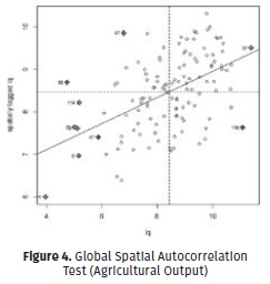
The Moran test is significant, rejecting the null hypothesis of no spatial autocorrelation. After this, we can continue with our spatial analysis, claiming a dependence between geographical units (municipalities) that decreases as the distance increases (Chasco, 2003). The autocorrelation is generally positive, and this pattern of interaction can be defined as an adjacency effect (Osland, 2010).
Often, in similar applications of spatial econometrics, what seemingly excels as spatial autocorrelation can respond to a missing explanatory variable such as the emergence of an economic subcenter (Osland, 2010), and this is the reason why spatial autocorrelation in the main variable deserves a further investigation.
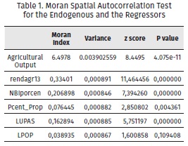
In the Table 1 appears the description of the spatial patterns for each variable used during the econometric strategy. The Moran tests applied to each regressor indicate the type of spatial distribution in space. Depending on the spatial behavior, the variables may be clustered or scattered in space. The null hypothesis states that there is no evidence of spatial autocorrelation across geographic units. In most of the tests, the null hypothesis of no spatial effects must be rejected at very stringent confidence levels.
The results of the significance tests indicate that all variables, except the log of population, show spatial autocorrelation. In the case of the log of the population, there is no evidence of spatial autocorrelation because the high values of the population are scattered throughout the territory. The main municipalities appear to be scattered with no clear spatial pattern.
Bernat (1996) runs regressions using the OLS procedures and later, in three separated models, he submits data to standard correction of spatial autocorrelation, either by a lag model or by a spatial error model. Applying three different contrasts, he finds strong evidence about the presence of spatial autocorrelation and once correction is applied, his results contribute to a better fit of the model.
In the first model of substantial spatial autocorrelation, spatial lag must be assumed as an endogenous variable and a suitable method must be applied, considering that the OLS (Ordinary Least Squares) model offers biased and inconsistent estimators (Anselin 2001). In the second model, when spatial interaction is identified as a spatial error type, estimators are inefficient and, in consequence, statistical inference is invalid although it could be unbiased (Helsen, 2008). On the other hand, in the case of substantive spatial autocorrelation, estimations will be biased and inconsistent even if the error term is not correlated (Moreno & Vayá, 2002).
Dubin (1998) insists on a careful handling when spatial autocorrelation is detected, because the presence of spatial autocorrelation has important implications in the context of the regression model. This situation is almost ubiquitous when data are distributed in space or when location is a fundamental criterion. In this case the classical OLS regressors turn out in unbiased but inefficient estimators and the variance of estimators is biased as well.
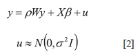
The OLS estimation does not incorporate spatial effects, and consequently it has no big relevance, although it is used as a benchmark for comparison with the remaining models. Such a non-spatial linear regression model is defined as:

where Y is an n x 1 vector of observations of the dependent variable associated with each spatial unit (k=1,..., N), lN corresponds to an n x 1 vector of ones associated with constant parameters α, X a n x K matrix representing exogenous variables with the set of associated parameters β and εi as an independent and identically distributed error term for all i, with zero mean and variance σ2.
Based on the previous consideration, any correction of autocorrelation contributes to obtaining more accurate estimates and to improving the reliability of the hypothesis test. When the structure of the autocorrelation is estimated, its information is incorporated into the prediction to improve accuracy. To do this, maximum likelihood (ML) techniques are commonly used to model the autocorrelation parameters and estimate the regression (Dubin, 1998).
At the beginning of the spatial analysis, we need to define an interaction structure represented by the matrix W, which represents the exogenous spatial weights that impose the assumed spatial dependence between the observations.
The presence of spatial autocorrelation in the regression model can be explained in two ways: it is possible that exogenous or endogenous variables be correlated spatially or that error term have an autocorrelation scheme (Moreno & Vayá, 2002).
In the first case, it is necessary to specify the following model:
In equation (1) it can be observed that if spatial lag is omitted in exogenous or endogenous variables, the feature of spatial dependence will be transmitted to the error term, in the case quoted as substantive spatial autocorrelation. In facing this situation, it is necessary to include the spatial lag of the variable within the spatial autocorrelation.
These models are also known as Models of Communication or Contagion and integrate the whole autocorrelation structure into spatial lag as an explicative argument of the endogenous variable. In the case of omission of weight matrix in this type of a model, estimation commits a specification error that biases estimators and leads to invalid inference (Moreno & Vayá, 2002).
In the second case, if spatial autocorrelation is present only in the error term, the model to be estimated corresponds to:
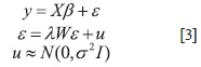
Where u is a white noise term and λ becomes the autoregressive parameter. It means that we incorporate an autoregressive process in the error terms and consider that ξ, is related not only to a stochastic term of error, but it is also a function of non-included exogenous variables of neighboring places and therefore there are several omitted variables spatially correlated to one another.
In equation 3, if there is no omission of the lag in the variables of the model, it corresponds to the case spatial autocorrelation of the residuals, and then a scheme of spatial dependence in the error term must be included (Moreno & Vayá, 2002). In the implementation of the spatial error model, we assume that there is an autoregressive process in the error terms, and we assume that there is some kind of spillover effect on the residuals.
As usual in the practice of spatial econometrics the OLS model barely has informative purposes, but it is not considered due to a potential bias. In fact, when there is evidence about spatial autocorrelation in the dependent variable and this feature is not modeled, OLS estimates the result to be biased and inconsistent (Anselin, 2001). Typically, in the spatial analysis inconsistency emerges by the multidirectional dependency in the data, taken into account when comparing the widely known autocorrelation related to time series and the spatial autocorrelation.
In spatial econometrics, the maximum likelihood is commonly used since the autoregressive parameter must be estimated simultaneously with the other parameters (Osland, 2010). In fact, the standard treatment of econometrics in presence of spatial autocorrelation runs a regression via maximum likelihood. As it is known in this technique, regressors are calculated maximizing the logarithm of the likelihood function associated with the spatial model (Moreno & Vayá, 2002).
We apply an additional perspective. Elhorst (2010), following LeSage's suggestion, applies an innovative model with an endogenous spatially lagged variables and, in addition, the lag structure of all exogenous variables, under the assumption that the behavior of neighbors globally affects the model under estimation. In the latter case, we estimate direct and indirect effects that are represented by the respective coefficient of the contemporaneous spatial effect, and the lagged influence of the exogenous variable belonging to neighboring spaces. Such a procedure is widely referred to as the spatial Durbin model, and its specification corresponds to the following model:
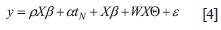
where ε=(εi,..., εN) is a vector of disturbances, in which ei are error terms distributed independently and identically with 0 mean and variance σ2.
The Durbin model is defined assuming a spatial lag of the dependent variable, alongside a spatial lag of all exogenous variables. The last one purports to capture effects as described for the attributes of the conterminous municipalities influencing the output in each geographical unit. The Durbin model is composed to provide a neighboring output to determine local production, simultaneously to the characteristics of conterminous spaces (Osland 2010).
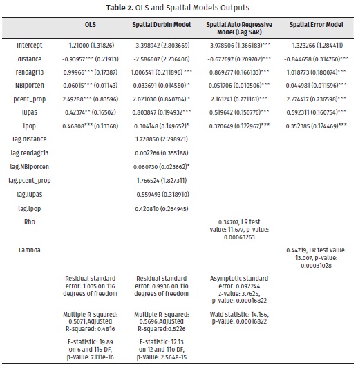
In Table 2, regarding the lag model, the parameter rho is significant indicating a spatial dependence on the local output, influenced by the values in conterminous municipalities, seemingly sharing similar geographical and production conditions. As already mentioned, the statistical characteristics of both models are similar although each one leads to a different final interpretation. In the lag model, a rho parameter appears that indicates the magnitude of the effect of neighboring units on the endogenous variable.
The parameter rho is referred to as the spatial correlation or spatial dependence parameter, which appears in equation (2) and indicates the intensity of the dependence between adjacent agricultural outputs. If a non-significant value of rho is assumed, the observed spatial structure is not representative (Osland, 2010). Regarding the exogenous variables, all of them demonstrated to be significant.
The statistically significant spatial error coefficient (rho) suggests that the autocorrelation may be due to the fact that the data are aggregated on the basis of municipal boundaries, which have a political but no economic meaning. The statistically significant spatial lag coefficient suggests that a local output is significantly affected by the productive relevance of its conterminous areas.
On the other hand, focusing on the spatial error process and according to the Table 2, the comparison between the OLS model and the spatial error model reveals an encouraging conclusion in the sense that there are no drastic changes in the regressors in terms of mathematical sign and significance. It is a proof that the information contained in the errors is not mainly due to omitted variables, and that there are small and imperceptible exogenous and unexplained spatial interaction processes that decrease as the distance between spatial units increases (Osland, 2010).
When the structure of autocorrelation is assumed in the residuals (spatial error model), we must specify a spatial autoregressive model in pursuing the improvement in the estimates. With this structure, we insert the most relevant determinants in the model, relegating the subtler spatial information to the residuals (Osland, 2010).
In both spatial error and spatial lag, all the arguments explaining the output are significant, demonstrating the correct choice of exogenous variables, and the remarkable relevance of the model specification. The distance to Bogotá, however, reveals a counterintuitive result, perhaps because the distance is measured as a linear distance, ignoring the stubborn precariousness of the roads, and the intricate connections in the most remote places. We should expect that spatial barriers can hinder the possibilities of interaction in some spatial units each other (Osland, 2010), and we can assume that some transport costs come along as a relevant determinant in the economic interactions.
The arguments describing the rural conditions (Unsatisfied Basic Needs [UBN] and ownership) have positive coefficients highlighting poverty, which critically affects the rural sector in the five dimensions of the poverty indicator (UBN). The results also emphasize that the production drivers are not sufficient for dragging the producers out of poverty, and that public policy interventions are required to improve the conditions in the rural milieu. The backwardness predominates in the rural sector, considering that there is a kind of a relative poverty bias, which becomes a relevant factor in the analysis, given that 42% of Boyacá's population lives in the rural sector (CGIAR, 2021).
The proportion of owners and the number of rural exploitations (APUs) reinforce the output, because Boyacá is typically a region of small exploitations conducted by farmers and their families, amid a forcefully fragmented structure of land.
Finally, the local population is also highly significant demonstrating the role of the local pool of inhabitants as the main market for smallholder production, but also revealing its role as a source of labor input for the agricultural production process. This evidence is relevant for linking the familiar quality of the rural production and the demarcation of rural neighbor markets. The intuition that housing and labor markets are spatially self-contained (Osland 2010) can be applied in this analysis, due to the lack of dynamic labor markets and the limited mobility for rural workers.
The geographical variable that measures the distance to Bogotá from all the municipal centroids has a sign that is counter-intuitive, although the estimates are significant. This could be contrary to the hypothesis that asserts some kind of gravitational principle. The reason for the sign of a coefficient could be the inclusion of a linear distance, which does not measure the roughness of the terrain and the real cost of transport, or the existence of coexisting regional sub-centers of demand (Tunja, Sogamoso), whose distance measurements are not included in the analysis, although they are relevant for certain goods.
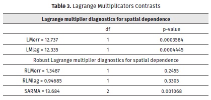
Upon performing the Moran's I test and rejecting the null hypothesis of absence of spatial effects, we proceed to run the Lagrange multiplier (LM) tests. Typically, two main variants of these LM-tests are applied in the analysis.
The first one is the LM-lag statistic test stating the null hypothesis of absence of spatial autocorrelation in the dependent variable (Baysoy 2023). On the other hand, the LM-error statistic test plays with the null hypothesis about the absence of significant spatial error autocorrelation. When both hypotheses are rejected, the decision criterion for choosing the suitable model considers which value of the test statistics is the largest and the most significant (Osland, 2010).
According to the Lagrange multiplier criteria, the error model is the more appropriate specification to describe the spatial dependence, so the local output in each municipality is strongly influenced by the values of the same variable in the conterminous areas. In this context, the high magnitude of agricultural output corresponds to common production advantages shared by conterminous municipalities.
The Lagrange multiplier (LM) statistic for spatial error is statistically significant, indicating that this is the specification of choice to deal with autocorrelation. Osland (2010) points out that the LM-error test over-rejects the null hypothesis in the presence of heteroscedasticity, and the LM-lag statistic is more robust, consistently with our decision criterion which recommends us the spatial lag model. Accordingly, in our procedure the results from the LM-lag tests hence give us more confidence. Then, the influence originated in neighbor entities affects local values if a variable in nearer places deviates strongly from the expected value (Bernat, 1996). This decision criterion according to the Lagrange multiplier diagnostic is crucial for determining whether the structure of spatial dependence relies on the nuisance, or on the structure of spatial units themselves (Suescún, 2013).
Regarding the information at the bottom of Table 6 the usefulness of robust LM contrast relies on the fact that the RLM-error test performs an adjustment for the presence of local spatial lag dependence, whereas the LM-error test takes for granted the absence of this kind of autocorrelation. In the spatial lag assessment, the RLM-lag statistic tests the null hypothesis that rho is zero, adjusting for the presence of local spatial error dependence (Osland, 2010).
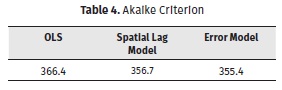
In order to reinforce the conclusion provided by the Lagrange multiplier criteria we conducted the process to estimate the Akaike criterion, and in fact it validated the choice of the spatial error model, taking as reference the lower value of the criterion. Accordingly, we are supported to assert the existence of common stochastic shocks affecting the agricultural output, across the wide set of geographical units. Such common influences are derived from the improvement of infrastructures, the diffusion of public policies or climate impacts. The Akaike criterion is used to elucidate the most appropriate spatial structure, in this case spatial autoregressive spatial model (Osland, 2010).
CONCLUSIONS
In terms of agricultural production, Boyacá has maintained its specialization in annual crops, despite the national trend of growth in the perennial crops. Except for sugarcane and some fruits in the milder areas, the main regional products are potatoes, onions and tomatoes, typically produced on cold lands. The share of exports is still insignificant compared to the total production, and most of the production is intended to meet the national consumption.
Accordingly, the structure of land ownership is based on small production units, whose availability of labor force depends on the family supply. The scale of production on small farms is low, and the technological modernization is therefore expensive in a such condition. Restricted access to technology in the rural sector reveals long-standing institutional and market failures that impede the modernization of small units.
The stubborn hypothesis of the "inverse relationship" corresponds to the typical structure of the rural sector in Boyacá, in terms of the fragmentation and small size of the farms. However, there is a huge challenge to increase the productivity of labor and endowment, which are ultimately the main constraints to the modernization the rural sector. Increasing the Total Factor Productivity of factors is a prerequisite for coping with the landslide of imports, specifically corns, wheat and barley.
According to Suescún (2013), the macro-transformation in Colombian agriculture towards a more extensive focus on perennial crops, harnesses the expansion of technical improvements to such extent, that the ultimate purpose of this tenure of land is the ownership itself, but not the technology nor the knowledge. However, this assertion is not fully valid as in big agribusiness units the application of technology looms as highly profitable, bearing in mind the exploitation of economies of scale, and the powerful underpinning for expanding investment and mechanization.
The role of Boyacá in the production of products to meet the domestic needs is relevant in a handful of products, namely: potatoes, onions, tomatoes and fruits. However, there is a timid emergence of exports of specific products demanded by niche markets abroad.
At the national level, the census revealed a process of demographic aging, and a growing relevance of female-headed households in the rural sector, amidst noticeable conditions of precariousness (Machado, 2015). According to the demographic trends, the process of rural depopulation is looming, although it can be contained by increasing agricultural profitability and sectoral modernization.
The spatial econometrics provided us with the evidence of an autoregressive spatial process in the error, asserting the action of common stochastic shocks reverberating the agricultural output across all municipalities.
ACKNOWLEDGMENTS
The authors are deeply thankful to the Masaryk Institute of High Studies at the Czech Technical University in Prague (Czech Republic), the Academy of Humanitas in Sosnowiec (Poland), and the College of Applied Psychology in the Czech Republic, by their stimulating academic support.
CONFLICT OF INTEREST STATEMENT
The authors declare that there is no conflict of interest.
FINANCIAL SUPPORT
The authors received no financial support for the research, authorship, and/or publication of this article.
NOTES
1 Coffee, sugar cane, cane, oil palm, cotton, rubber, tobacco, inter alia.
2 Departamento Administrativo Nacional de Estadística.
3 Instituto Geográfico Agustín Codazzi.
REFERENCES
[1] Anselin, L. (2001). Spatial Econometrics. In B. Baltagi (ed.), Companion to Theoretical Econometrics (pp. 310-330). Blackwell Publishing.
[2] Arbia, G. (2001). Modelling the Geography of Economic Activities on a Continuous Space. Papers in Regional Science, 80, 411-424. http://dx.doi.org/10.1007/PL00013646
[3] Arbia, G, Espa, G & Quah, D. (2008). A Class of Spatial Econometrics. Empirical Economics, 34(1), 81-103.
[4] Barrett, C., Bellemare, M. & Hou, J. (2010) Reconsidering Conventional Explanations of the Inverse Productivity-Size Relationship. World Development, 38(1), 88-97. http://dx.doi.org/10.1016/j.worlddev.2009.06.002
[5] Baysoy, M. (2023). Regional Growth Model with Spatial Externalities. In H. Arias & G. Antosova (eds.), Considerations of Territorial Planning, Space, and Economic Activity in the Global Economy. IGI Global. http://dx.doi.org/10.4018/978-1-6684-5976-8
[6] Bernat, A. (1996). Does Manufacturing Matter? A Spatial Econometric View of Kaldor's view. Journal of Regional Science, 36(3), 463-477.
[7] Berry, A. (2017), La agricultura familiar y la inclusión: un factor contribuyente a la paz. Revista Colombiana de Ciencias Pecuarias, 30, 9-12
[8] Chasco, C. (2003). Métodos gráficos del análisis exploratorio de datos espaciales. En Anales de economía aplicada. Asociación Española de Economía Aplicada.
[9] CGIAR. (2021). Análisis de oportunidades de mercado para productos agropecuarios de Boyacá, con potencialidad para reducir la emisión de carbono mediante una producción adaptada al clima. Documento de trabajo. Programa de Investigación de CGIAR en Cambio Climático, Agricultura y Seguridad Alimentaria
[10] DANE. (2014). Censo Nacional Agropecuario. Novena entrega de resultados 2014. DANE.
[11] Dubin, R. (1998). Spatial Autocorrelation: A Primer. Journal of Housing Economics, 7, 304-327. https://doi.org/10.1006/jhec.1998.0236
[12] Duranton, G. & Overman, H. (2005). Testing for Localization Using Micro-geographic Data. Review of Economic Studies, 72(4), 1077-1106. https://doi.org/10.1111/0034-6527.00362
[13] Elhorst, P. (2010). Applied Spatial Econometrics: Raising the Bar. Spatial Economic Analysis, 5(1). http://dx.doi.org/10.1080/17421770903541772
[14] Fedesarrollo. (2019). Uso potencial y efectivo de la tierra agrícola en Colombia: resultados del Censo Nacional Agropecuario. Fedesarrollo.
[15] Helsen, J. (2008). Essays on the Spatial Analysis of Manufacturing. In Ph. D. Dissertation, Ken State University. Graduate School of Management.
[16] Krugman P. (1992). Geografía y comercio. Antoni Bosch.
[17] Machado, A. (2015) El Censo Agropecuario: sorpresas o confirmaciones. Razón Pública. https://razonpublica.com/el-censo-agropecuario-sorpresas-o-confirmaciones/
[18] Moreno, R. & Vayá, E. (2002). Econometría espacial: nuevas técnicas para el análisis regional. Una aplicación a las regiones europeas. Investigaciones Regionales, (1), 83-106.
[19] Osland, L. (2010). An Application of Spatial Econometrics in Relation to Hedonic House Price Modeling. Journal of Real Estate Research, 32(3), 289-320. http://dx.doi.org/10.1080/10835547.2010.12091282
[20] Rojas, N. (2019). Determinantes de la productividad agrícola. Archivos de Macroeconomia, (500).
[21] Suescún, C. (2013) La inercia de la estructura agraria en Colombia: determinantes de la concentración especial de la tierra mediante un enfoque especial. Cuadernos de Economía, 32(61) 653-682.
[22] UNDP. (2011). Colombia rural. Razones para la esperanza. Informe Nacional de Desarrollo Urbano. https://www.undp.org/sites/g/files/zskgke326/files/migration/co/undp-co-ic_indh2011-parte1-2011.pdf